13.1. Jointly Distributed Pairs of Random Variables#
13.1.1. Code for 3-D Plots#
from matplotlib import pyplot as plt
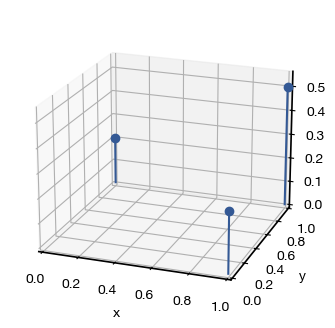
x = [1,0,1]
y = [0,1,1]
z = [1/4, 1/5, 1/2]
fig, ax = plt.subplots(subplot_kw=dict(projection='3d'))
ax.stem(x, y, z,basefmt=' ')
ax.view_init(20, azim = -70)
ax.set_xlabel('x')
ax.set_ylabel('y')
ax.set_ylim(0, 1)
ax.set_xlim(0, 1)
ax.set_zlim(0, 0.55);
import scipy.stats as stats
from matplotlib import cm
from matplotlib.ticker import LinearLocator, FixedLocator
import numpy as np

N=stats.multivariate_normal([0,0])

X = np.arange(-3, 3, 0.01)
Y = np.arange(-3, 3, 0.01)
X, Y = np.meshgrid(X, Y)
pos = np.dstack((X,Y))
Z=N.pdf(pos)


fig, ax = plt.subplots(subplot_kw={"projection": "3d"})


# Plot the surface.
surf = ax.plot_surface(X, Y, Z, cmap=cm.coolwarm,
                       linewidth=0, antialiased=False)

# Customize the z axis.
ax.set_zlim(0, 0.16)
ax.zaxis.set_major_locator(FixedLocator([0, 0.05, 0.10, 0.15]))
# A StrMethodFormatter is used automatically
ax.zaxis.set_major_formatter('{x:.02f}')


# Add a color bar which maps values to colors.
fig.colorbar(surf, shrink=0.5, aspect=5)

ax.view_init(35, azim = -120)
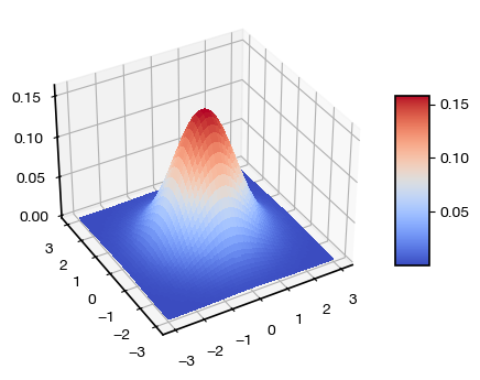
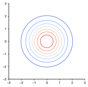
Contours of equal probability density for zero-mean, unit variance, independent Normal random variables
K1=np.array([
    [1,0],
    [0,1]
])

G = stats.multivariate_normal(mean=[0,0],cov=K1)


plt.figure( figsize=(4,4))
plt.contour(X,Y,G.pdf(pos), extent=[-3,3,-3,3], cmap=cm.coolwarm);
plt.xlim(-3,3)
plt.ylim(-3,3);
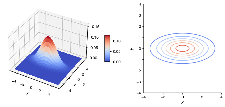
Surface plot of density and contours of equal probability density for zero-mean independent Normal random variables with \(sigma_{X}^2 =3\) and \(\sigma_{Y}^{2} = 0.5\)
N=stats.multivariate_normal([0,0],cov= np.array([[3, 0], [0,0.5]]))

X = np.arange(-5, 5, 0.01)
Y = np.arange(-5, 5, 0.01)
X, Y = np.meshgrid(X, Y)
pos = np.dstack((X,Y))
Z=N.pdf(pos)


from matplotlib import cm
from matplotlib.ticker import LinearLocator
import numpy as np

fig,axs = plt.subplot_mosaic('AAABB', figsize=(10,4))

ss = axs['A'].get_subplotspec()
axs['A'].remove()
axs['A'] = fig.add_subplot(ss, projection='3d')
ax=axs['A']


# Plot the surface.
surf = ax.plot_surface(X, Y, Z, cmap=cm.coolwarm,
                       linewidth=0, antialiased=False)

# Customize the z axis.
ax.set_zlim(0, 0.16)
ax.zaxis.set_major_locator(FixedLocator([0, 0.05, 0.10, 0.15]))
# A StrMethodFormatter is used automatically
ax.zaxis.set_major_formatter('{x:.02f}')


# Add a color bar which maps values to colors.
fig.colorbar(surf, shrink=0.3, aspect=5, pad=0.1)

ax.view_init(35, azim = -60)
ax.set_xlabel('$x$');
ax.set_ylabel('$y$');

ax=axs['B']
#ax = fig.add_subplot(1,2,2)
# #G = stats.multivariate_normal(mean=[0,0],cov=K1)


ax.contour(X,Y,N.pdf(pos), extent=[-3,3,-3,3],cmap=cm.coolwarm);
ax.set_ylim(-4,4)
ax.set_xlim(-4,4);
ax.set_xlabel('$x$');
ax.set_ylabel('$y$');
# ax.spines['bottom'].set_position('zero')
# ax.spines['left'].set_position('zero')
plt.subplots_adjust(wspace=0.7)
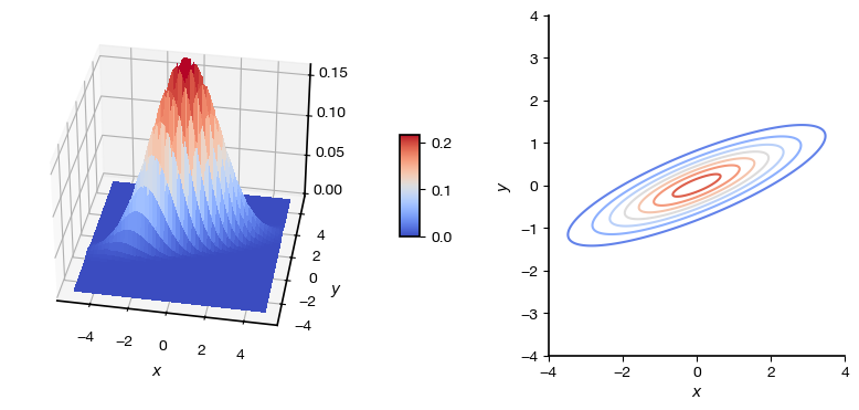
Surface plot of density and contours of equal probability density for zero-mean Normal random variables with \(sigma_{X}^2 =3\), \(\sigma_{Y}^{2} = 0.5\), and \(\rho =0.82\)
N=stats.multivariate_normal([0,0],cov= np.array([[3, 1], [1,0.5]]))

X = np.arange(-5, 5, 0.01)
Y = np.arange(-5, 5, 0.01)
X, Y = np.meshgrid(X, Y)
pos = np.dstack((X,Y))
Z=N.pdf(pos)


from matplotlib import cm
from matplotlib.ticker import LinearLocator
import numpy as np

fig,axs = plt.subplot_mosaic('AAABB', figsize=(10,4))

ss = axs['A'].get_subplotspec()
axs['A'].remove()
axs['A'] = fig.add_subplot(ss, projection='3d')
ax=axs['A']


# Plot the surface.
surf = ax.plot_surface(X, Y, Z, cmap=cm.coolwarm,
                       linewidth=0, antialiased=False)


# Customize the z axis.
ax.set_zlim(0, 0.16)
ax.zaxis.set_major_locator(FixedLocator([0, 0.05, 0.10, 0.15]))
# A StrMethodFormatter is used automatically
ax.zaxis.set_major_formatter('{x:.02f}')


# Add a color bar which maps values to colors.
fig.colorbar(surf, shrink=0.3, aspect=5, pad=0.1)

ax.view_init(35, azim = -80)
ax.set_xlabel('$x$');
ax.set_ylabel('$y$');

ax=axs['B']
# #G = stats.multivariate_normal(mean=[0,0],cov=K1)


ax.contour(X,Y,N.pdf(pos), extent=[-3,3,-3,3],cmap=cm.coolwarm);
ax.set_ylim(-4,4)
ax.set_xlim(-4,4);
ax.set_xlabel('$x$');
ax.set_ylabel('$y$');
# ax.spines['bottom'].set_position('zero')
# ax.spines['left'].set_position('zero')
plt.subplots_adjust(wspace=0.7)
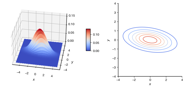
Surface plot of density and contours of equal probability density for zero-mean Normal random variables with \(sigma_{X}^2 =3\), \(\sigma_{Y}^{2} = 0.5\), and \(\rho =-0.3\)
cov = (-0.3) *np.sqrt(3)*np.sqrt(0.5)
N=stats.multivariate_normal([0,0],cov= np.array([[3, cov], [cov,0.5]]))

X = np.arange(-5, 5, 0.01)
Y = np.arange(-5, 5, 0.01)
X, Y = np.meshgrid(X, Y)
pos = np.dstack((X,Y))
Z=N.pdf(pos)


from matplotlib import cm
from matplotlib.ticker import LinearLocator
import numpy as np

fig,axs = plt.subplot_mosaic('AAABB', figsize=(10,4))

ss = axs['A'].get_subplotspec()
axs['A'].remove()
axs['A'] = fig.add_subplot(ss, projection='3d')
ax=axs['A']


# Plot the surface.
surf = ax.plot_surface(X, Y, Z, cmap=cm.coolwarm,
                       linewidth=0, antialiased=False)


# Customize the z axis.
ax.set_zlim(0, 0.16)
ax.zaxis.set_major_locator(FixedLocator([0, 0.05, 0.10, 0.15]))
# A StrMethodFormatter is used automatically
ax.zaxis.set_major_formatter('{x:.02f}')


# Add a color bar which maps values to colors.
fig.colorbar(surf, shrink=0.3, aspect=5, pad=0.1)

ax.view_init(35, azim = -80)
ax.set_xlabel('x');
ax.set_ylabel('y');

ax=axs['B']
# #G = stats.multivariate_normal(mean=[0,0],cov=K1)


ax.contour(X,Y,N.pdf(pos), extent=[-3,3,-3,3],cmap=cm.coolwarm);
ax.set_ylim(-4,4)
ax.set_xlim(-4,4);
ax.set_xlabel('x');
ax.set_ylabel('y');
# ax.spines['bottom'].set_position('zero')
# ax.spines['left'].set_position('zero')
plt.subplots_adjust(wspace=0.7)
13.1.2. Terminology Review#
Use the flashcards below to help you review the terminology introduced in this chapter. \(~~~~ ~~~~ ~~~~ \mbox{ }\)