3.4. Summary Statistics

Self-Assessment:

The following questions can be used to check your understanding of the material covered in this chapter: \(~~ \!\!\)

Terminology Review

Use the flashcards below to help you review the terminology introduced in this section. \(~~~~ ~~~~ ~~~~ \mbox{ }\)

3.4.1. Code for Figures

Here is the code to generate Figures 3.1 and 3.2 in Foundations of Data Science with Python:

import matplotlib.pyplot as plt
import numpy as np

# For clarity, store the different error metrics in different variables.
# Initialize them here
sum_errors = 0
num_nonzero_errors = 0
sum_abs_errors = 0
sum_square_errors = 0

nus = np.arange(-2, 6.01, 0.01) 
D = [-1, -1, 0, 2, 5]

# Calculate the error metrics
for d in D:
    sum_errors += d - nus
    num_nonzero_errors += np.round((d - nus),10) != 0
    sum_abs_errors += np.abs(d - nus)
    sum_square_errors += (d - nus) ** 2

# Plot the error metrics as a function of the summary statistic, v
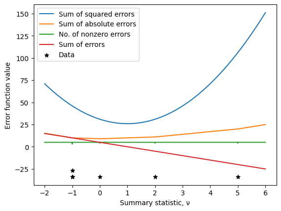
plt.plot(nus, sum_square_errors, label="Sum of squared errors")
plt.plot(nus, sum_abs_errors, label="Sum of absolute errors")
plt.plot(nus, num_nonzero_errors, label="No. of nonzero errors")
plt.plot(nus, sum_errors, label="Sum of errors")

# Plot the data as markers
ymin, ymax = plt.ylim()
plt.scatter(D, ymin * np.ones(5), marker="*", label="Data", color="k")
# Plot the repeated value at -1 as a second marker:
plt.scatter(D[0], ymin + 7, marker="*", color='k')

plt.xlabel(r"Summary statistic, ν")
plt.ylabel("Error function value")
plt.legend();

nu_e = nus[np.argmin(sum_errors)]
nu_0 = nus[np.argmin(num_nonzero_errors)]
nu_1 = nus[np.argmin(sum_abs_errors)]
nu_2 = nus[np.argmin(sum_square_errors)]


print("         Metric         |     Minimizing value of nu")
print("____________________________________________________")
print(f'{"Sum of errors": ^24s}|{np.round(nu_e):^30}')
print(f'{"No. nonzero errors": ^24s}|{np.round(nu_0):^29}')
print(f'{"Sum of abs errors": ^24s}|{np.round(nu_1):^30}')
print(f'{"Sum of squared errors": ^24s}|{np.round(nu_2):^30}')

         Metric         |     Minimizing value of nu
____________________________________________________
     Sum of errors      |             6.0              
   No. nonzero errors   |            -1.0             
   Sum of abs errors    |             0.0              
 Sum of squared errors  |             1.0              

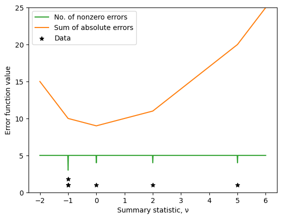
nus = np.arange(-2, 6.01, 0.01) 
D = [-1, -1, 0, 2, 5]
# For clarity, store the different error metrics in different variables.
# Initialize them here
num_nonzero_errors = 0
sum_abs_errors = 0

# Calculate the error metrics
for d in D:
    num_nonzero_errors += np.round((d - nus),10) != 0
    sum_abs_errors += np.abs(d - nus)

plt.plot(nus, num_nonzero_errors, label="No. of nonzero errors", color= 'C2')
plt.plot(nus, sum_abs_errors, label="Sum of absolute errors", color='C1')

# Plot the data as markers
plt.ylim(0, 25)
ymin = 1
plt.scatter(D, ymin * np.ones(5), marker="*", label="Data", color="k")
# Plot the repeated value at -1 as a second marker:
plt.scatter(D[0], ymin + 0.8, marker="*", color="k")


plt.xlabel(r"Summary statistic, ν")
plt.ylabel("Error function value")
plt.legend();